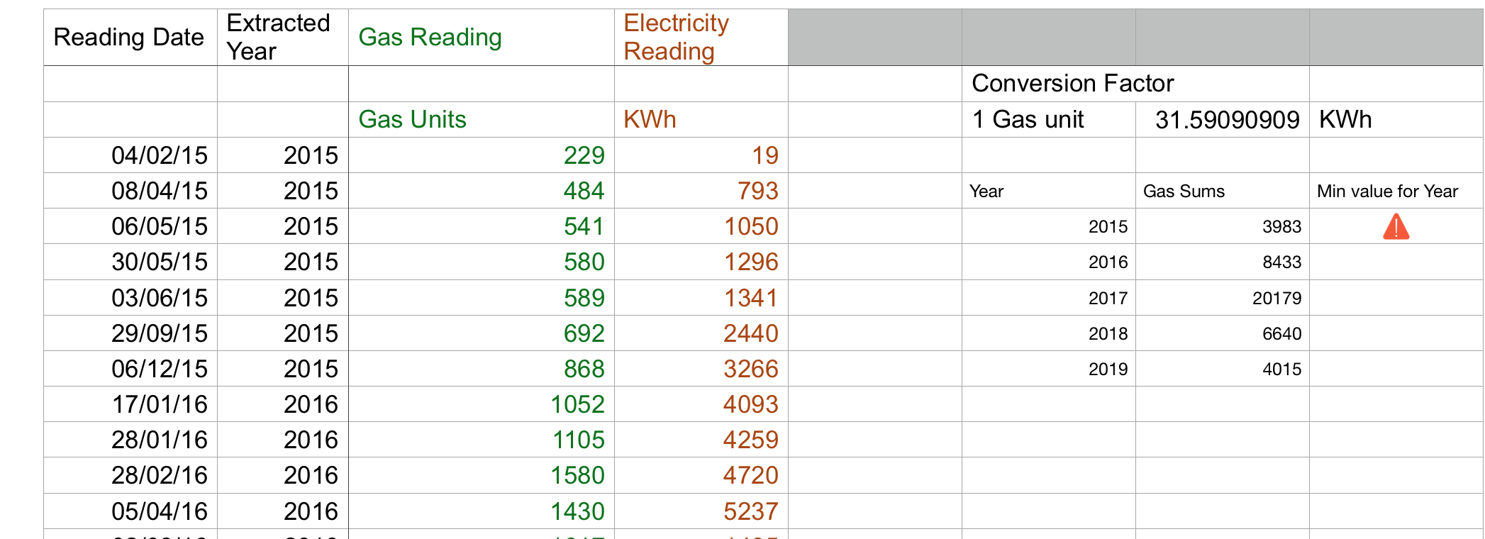
Presumably you mean that you want to compare each entry of B, so first you need to correct your SUMIF command to have a B:B rather than B.
SUMIF(B:B,...)
That will indicate the full B column.
However you seem to have the good idea of looking at the max and min readings on in 2015. In this case, you want to find a maximum among a range. In excel this is secretly doing two things: first, finding which cells happen to equal 2015 and picking those out. Then, find their maximum. To get the values for the Gas Reading when the year is 2015, you create a vector or "array" of values that are only the Gas Readings you want. This is the output of an if statement:
IF(B:B=F6,C:C)
which has the effect of looking at each entry of the B column, asking if it's equal to F6. If so, then return the corresponding element of the C column. Notice that it spits out a bunch of numbers not just one, so you can't just enter that expression above and see all the numbers. It's not a "function" (with one output).
You want the maximum of these numbers, minus the minimum of the same numbers, to get the amount of gas you used.
Therefore the function you seek is
=MAZ(IF(B:B=F6,C:C))-MIN(IF(B:B=F6,C:C))
Caveat!! Make sure to use control-shift-return. After you enter the formula, while your cursor is still in the function box, press "control-shift-return" rather than just return. This allows excel to deal with the array, i.e. all those values inside the max() function, all at once.

