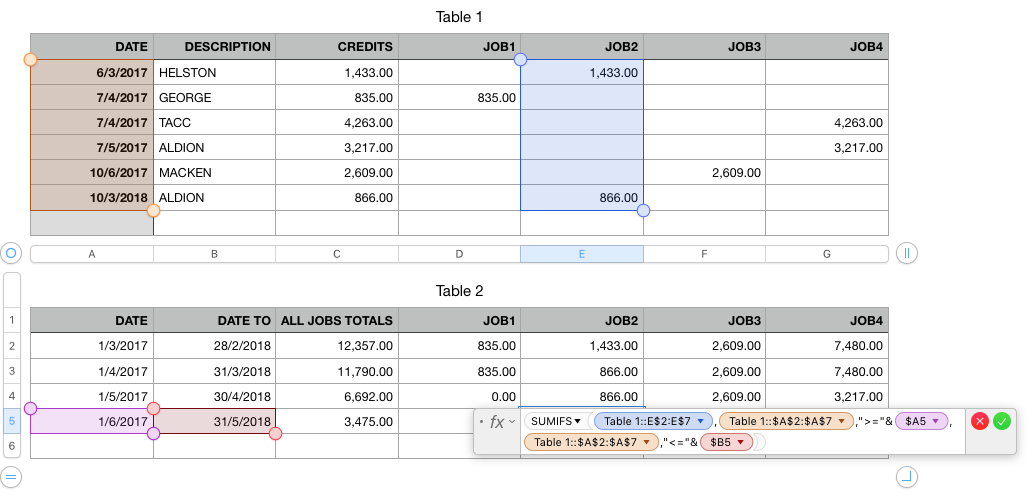
You can do this using the SUMIFS() function. The picture below shows how to do it using this function based on the samples of the input data table and the outcome table you have shared. Pls pay attention to the absolute references in the formula, i.e. the "$" signs; they are necessary for the formula to work correctly when you copy & paste it to other cells.
If you have any difficulty in creating the formula in cell E5 based on the picture below alone, you can recreate it by typing its following form in any cell appropriate (or simply copy & pasting it from this post).
= SUMIFS(Table 1::E$2:E$7,Table 1::$A$2:$A$7,">="&$A5,Table 1::$A$2:$A$7,"<="&$B5)
Note, however, if your actual input data table is placed differently (the one in the example I gave, including the header row, starts from A1) or bigger than the one in the example I gave, you would need to change some or all of the cell references in the example formula I give here.

