Lookup up cell values in Numbers

Question

I want to build a simple word translator which may look like this:

• COLUMN A: I have a list of words, each on a row. (1:Airplane, 2:Car, 3:Cat, 4:Dog etc..)
• COLUMN B: I have a list of the same words in another language, each on a row. (1:Aereoplano, 2: Macchina, 3:Gatto, 4:Cane etc..)

• Then I have two cells. In the first one, I can type any word. The second cell is the formula that I want to create. The formula should:

  • check if "my word"(the word that I type) is in the list of column A
  • if it exists, it should return its adjacent word of the second column
  • If no words match, the formula should not return anything.

I'm struggling with finding the correct functions to accomplish this, any pointers are welcome.

UPDATE I finally found the solution. Best solution for me is
=IFERROR(VLOOKUP(B7;'Table 1-1'::B4:D53;3;FALSE);0)
REALLY thanks for your help.

Answer 1

This answer to a related question explains how to use VLOOKUP in combination with IFERROR.

If VLOOKUP cannot find the exact match, then it throws an error. To catch this error, wrapping the formula in the IFERROR function allows the author to supply a default (in the OP's case, an empty string "") to display in the event of no match.

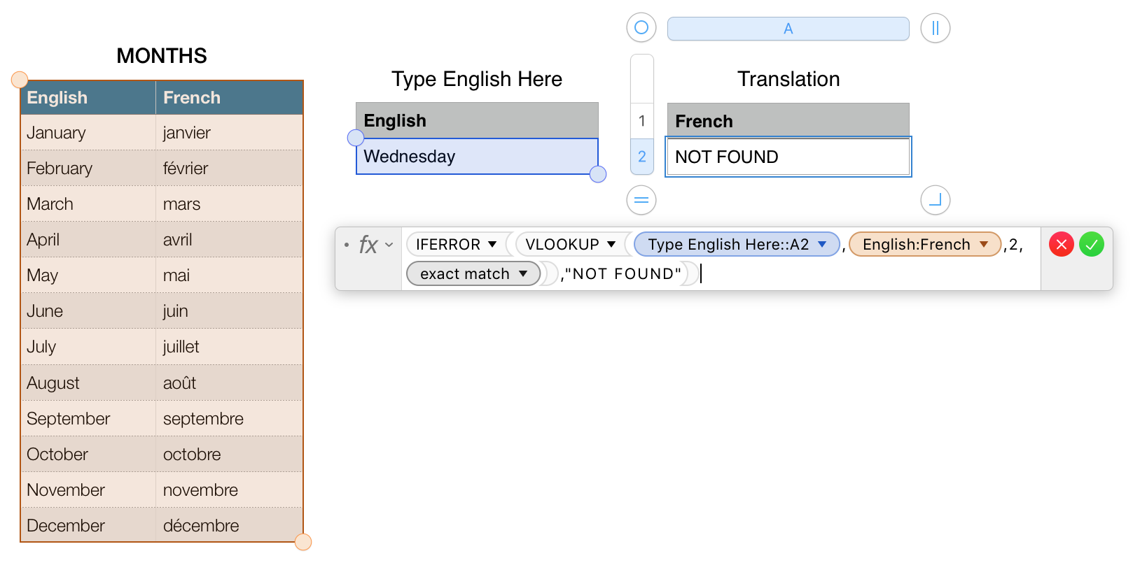
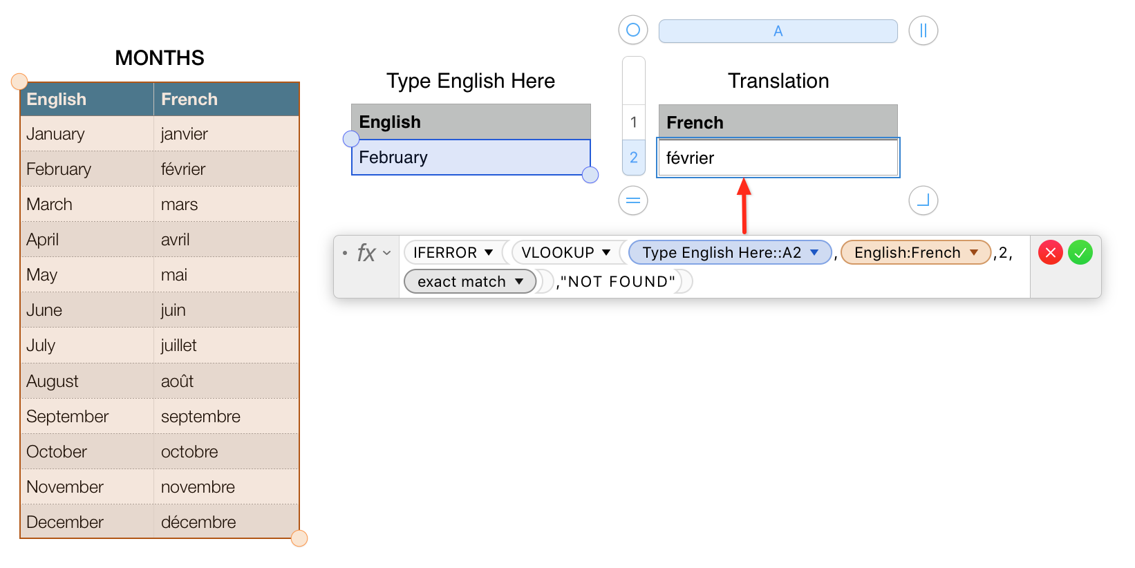
The following example uses a third table to display the translation. That table is then locked so as to protect the formula from being inadvertently overwritten. The words NOT FOUND are used here to show the error event.

If match is found:

No match:

From the documentation:

VLOOKUP(search-for, columns-range, return-column, close-match)

search-for: The value to find. search-value can contain any value.

columns-range: A collection of cells. columns-range must contain a reference to a single range of cells, which may contain any values.

return-column: A number value that specifies the relative column number of the cell from which to return the value. The leftmost column in the collection is column 1.

close-match: An optional modal value that determines whether an exact match is required.

close match (TRUE, 1, or omitted): If there’s no exact match, select the row with the largest left-column value that is less than or equal to the search value. If you use close match, you can’t use wildcards in search-for.

exact match (FALSE or 0): If there’s no exact match, returns an error. If you use exact match, you can use wildcards in search-for. You can use the wildcard ? (question mark) to represent one character, an * (asterisk) to represent multiple characters, and a ~ (tilde) to specify that the following character should be matched rather than used as a wildcard.